Zymplectic — Numerical tools for Hamiltonian systems

Introduction

A Hamiltonian describes a system through a single function that is often its total energy.

For a separable system, the Hamiltonian H is written as the sum of kinetic energy T, which depends on momentum p, and potential energy V, which depends on position q.

\[ H(q,p) = T(p) + V(q) \]

In plain language: the system’s state is split into a momentum part and a position part.

Hamilton’s equations connect those two coordinates. Momentum changes in response to the slope of the energy with respect to position; position changes in response to its slope with respect to momentum.

\[ \begin{aligned} \dot{p} &= -\frac{\partial H}{\partial q}, \\[4pt] \dot{q} &= \frac{\partial H}{\partial p}. \end{aligned} \]

A splitting method advances the state through a sequence of small substeps. At stage i, it first updates position and then momentum:

\[ \begin{aligned} q_i &= q_{i-1} + \tau c_i \frac{\partial T}{\partial p}\!\left(p_{i-1}\right), \\[6pt] p_i &= p_{i-1} - \tau d_i \frac{\partial V}{\partial q}\!\left(q_i\right). \end{aligned} \]

Here, τ is the time step; c_i and d_i are splitting coefficients; and the number of coefficient pairs determines the number of stages. Their values determine the splitting method’s order and accuracy.

Unlike a general-purpose Runge-Kutta methods, a symplectic integrator preserves the geometry of phase space. The energy is generally not perfectly constant at every step; instead, the energy error tends to remain bounded and oscillatory over long integrations. This behavior is especially valuable in celestial mechanics, accelerator physics, molecular dynamics, and quantum chemistry.

Zymplectic energy error display — Relative energy error as a function of time for the Hénon-Heiles system, a double pendulum and a gyro wheel. The energy is conserved over long simulations.

Extended applications

The cleanest case is autonomous and separable, but related techniques can also treat systems whose kinetic or potential energy changes explicitly with time:

\[ H(q,p,t) = T(p,t) + V(q,t) \]

These are non-autonomous systems, so the Hamiltonian need not be conserved. More advanced formulations extend the same splitting to non-separable systems, where position and momentum cannot be isolated into independent terms:

\[ H(q,p,t) = f(p,q,t) \]

With care, the same computational patterns can also be useful for differential equations that are not governed by a Hamiltonian, although some symplectic guarantees may no longer apply.

The Zymplectic project

Zymplectic differs from broad differential-equation libraries such as GSL or JuliaDiffEq: it is intentionally focused on Hamiltonian systems and explicit symplectic integrators.

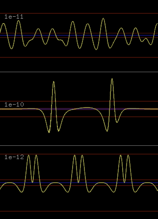
The application loads C/C++ source files containing Hamilton’s equations, compiles them, and runs the resulting model with the chosen method, visualisation, and numerical settings. It can present simulated objects, trajectories, energy surfaces, and error data without requiring users to learn a large application interface.

The downloadable package includes either MinGW GCC or Clang, so it can work without a separate IDE or compiler installation. The included MinGW are replacable with other and possibly newer builds of GCC or Clang.

Zymplectic's catalogue of numerical methods ranges from simple symplectic Euler and leapfrog methods to high-order symplectic partitioned Runge–Kutta and Runge–Kutta–Nyström schemes, but includes also customized construction of higher order methods by Yoshida's composition method as well as formally unpublished techniques.

Dynamical systems

The 100 dynamical systems included in the 0.16.1 release, not including advanced and constrained systems.

Showcases

Showcase list last updated 2023.03.27

Ease of use

A model needs Hamilton’s equations, initial conditions, and a short initialisation function. Macro-augmented C++ keeps comprehensive systems compact while retaining native performance.

Example Minimal Hénon–Heiles model

#include "math.h"

const double lambda = 1.0;
double _q_init[] = {0.3, 0.0}; // position
double _p_init[] = {0.0, 0.4}; // momentum

double energy_H(Arg) {
    return lambda*q2*(q1@2 - q2@2/3.0)
         + 0.5*(q1@2 + q2@2 + p1@2 + p2@2);
}

void dH(Arg) {
    dq1 = q1 + lambda*2*q1*q2;
    dq2 = q2 + lambda*(q1@2 - q2@2);
    dp1 = p1;
    dp2 = p2;
}

void main() {
    Z.H(energy_H, dH, 0);
}

Objects can be paired with one another or assigned to separate kinetic and potential energies, making larger physical systems possible with relatively little model code. Or multiple objects can be applied to the same system:

Example extended Added custom graphics

...

double _q_init[] = {0.3, 0.0,  0.2, 0.0,  0.1, 0.0};
double _p_init[] = {0.0, 0.4,  0.0, 0.3,  0.0, 0.2};

void DrawFunc() {
	for (int i = 0; i < 3; ++i)
		draw.sphere(obj_q[i][0], obj_q[i][1], 0, 0.1); 
}

void IterFunc() {
	// print output?
}

void main() {
	Z.OnDraw = DrawFunc; //graphics event
	Z.OnIter = IterFunc; //iteration event
    Z.H(energy_H, dH, 0); //multiple objects
    Z.H(energy_H, dH, 1);
    Z.H(energy_H, dH, 2);	
}

While some native graphics are supported without code, custom graphics support a wide range of practical graphical functions that work for both 2D and 3D display.

Zymplectic interface showing a three-dimensional simulation and numerical controls — The interface combines a control panel GUI, a graphics display, and an output console (not shown).

Dynamical systems

Explicit symplectic integration

Introduction

Extended applications

The Zymplectic project

Dynamical systems

Showcases

Ease of use

Further reading