Zymplectic project
The double pendulum
The Hamiltonian of the double pendulum is derived with two approaches and different implementations are presented.
Available with Zymplectic v.0.1.4
The double pendulum is a simple dynamical system which exhibit rich chaotic behavior.
The implementations discussed here are symplectic in spite of symplectic integratores rarely being associated with simulations of the double pendulum because it is governed by a non-separable Hamiltonian.
The Hamiltonian is obtained in the following two sections where two different derivations and implementations are presented.
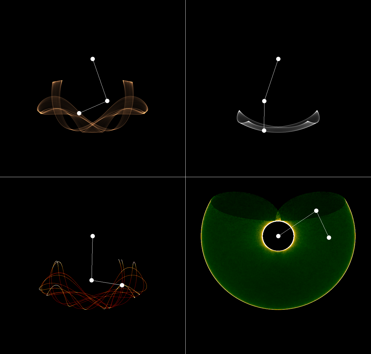
By defining the canonical coordinates as in the figure above, the cartesian coordinates of of the pendulum bob 1 and 2 can be expressed relative to the fixed pivot as:
The system is implemented as a non-separable system. Zymplectic automatically detects the system as non-separable because dp1,dp2..., dq1,dq2... and Z.H are used. The following code simulates the motion of the double pendulum:
It now follows that:
The double pendulum (method 1)
Define first the variables- l1 is the length of the pendulum from the fixed pivot to the first bob
- l2 is the length of the pendulum from the the pivot at the first bob to the bob of the second pendulum
- m1 and m2 are the masses of the first and second pendulum bob
- g is the gravitational constant
- q1 and q2 are the canonical coordinates associated with the pendulum angles (see image below)
- p1 and p2 are the canonical momenta
\(\displaystyle{\qquad x_1(t) = {l_1}\sin \left( {{q_1}} \right)}\)
\(\displaystyle{\qquad y_1(t) = {l_1}\cos \left( {{q_1}} \right)}\)
\(\displaystyle{\qquad x_2(t) = {x_1}\left( t \right) + {l_2}\sin \left( {{q_2}} \right)}\)
\(\displaystyle{\qquad y_2(t) = {y_1}\left( t \right) + {l_2}\cos \left( {{q_2}} \right)}\)
The velocities are obtained by differentiation:
\(\displaystyle{\qquad {{\dot x}_1}\left( t \right) = {l_1}{{\dot q}_1}\cos \left( {{q_1}} \right)}\)
\(\displaystyle{\qquad {{\dot y}_1}\left( t \right) = - {l_1}{{\dot q}_1}\sin \left( {{q_1}} \right)}\)
\(\displaystyle{\qquad {{\dot x}_2}\left( t \right) = {l_1}{{\dot q}_1}\cos \left( {{q_1}} \right) + {l_2}{{\dot q}_2}\cos \left( {{q_2}} \right)}\)
\(\displaystyle{\qquad {{\dot y}_2}\left( t \right) = - {l_1}{{\dot q}_1}\sin \left( {{q_1}} \right) - {l_2}{{\dot q}_2}\sin \left( {{q_2}} \right)}\)
The kinetic energy T and the potential energy V are expressed by the velocities and heights of the pendulum bobs:
\(\displaystyle{ \qquad T = \frac{1}{2}{m_1}\left( {\dot x_1^2 + \dot y_1^2} \right) + \frac{1}{2}{m_2}\left( {\dot x_2^2 + \dot y_2^2} \right) }\)
\(\displaystyle{ \qquad V = {m_1}g{y_1} + {m_2}g{y_2} }\)
Inserting positions and velocities yields:
\(\displaystyle{ \qquad T = {l_1}{l_2}{m_2}{{\dot q}_1}{{\dot q}_2}\cos \left( {{q_1} - {q_2}} \right) + \frac{1}{2}\left( {l_1^2\left( {{m_1} + {m_2}} \right)\dot q_1^2 + l_2^2{m_2}\dot q_2^2} \right) }\)
\(\displaystyle{ \qquad V = \left( {{m_1} + {m_2}} \right)g{l_1}\cos \left( {{q_1}} \right) + {m_2}g{l_2}\cos \left( {{q_2}} \right) }\)
The Lagrangian L = T - V is now known and utilized only to obtain the canonical momenta:
\(\displaystyle{ \qquad {p_1} = \frac{{\partial L}}{{\partial {{\dot q}_1}}} = {l_1}{l_2}{m_2}{{\dot q}_2}\cos \left( {{q_1} - {q_2}} \right) + l_1^2{{\dot q}_1}\left( {{m_1} + {m_2}} \right) }\)
\(\displaystyle{ \qquad {p_2} = \frac{{\partial L}}{{\partial {{\dot q}_2}}} = {l_1}{l_2}{m_2}{{\dot q}_1}\cos \left( {{q_1} - {q_2}} \right) + l_2^2{m_2}{{\dot q}_2} }\)
We desire to express the angular velocities in terms of the canonical coordinates and momenta. To achieve this, we solve the system of equations and obtain:
\(\displaystyle{ \qquad {{\dot q}_1}{l_1} = \frac{{{l_2}{p_1} - {l_1}{p_2}\cos \left( {{q_1} - {q_2}} \right)}}{{{l_1}{l_2}\left( {{m_2}{{\sin }^2}\left( {{q_1} - {q_2}} \right) + {m_1}} \right)}} }\)
\(\displaystyle{ \qquad {{\dot q}_2}{l_2} = \frac{{{l_1}{m_2}{p_2}\cos \left( {2{q_1} - 2{q_2}} \right) - 2{l_2}{m_2}{p_1}\cos \left( {{q_1} - {q_2}} \right) + {l_1}{p_2}\left( {2{m_2}\sin \left( {{q_1} - {q_2}} \right) + 2{m_1} + {m_2}} \right)}}{{2{l_1}{l_2}{m_2}\left( {{m_2}{{\sin }^2}\left( {{q_1} - {q_2}} \right) + {m_1}} \right)}} }\)
It follows from substitution of the angular velocity in the energies V and T that the energies are expressed only in terms of the canonical coordinates. After valiant simplifications, one obtains:
\(\displaystyle{ \qquad V\left( {{q_1},{q_2}} \right) = \left( {{m_1} + {m_2}} \right)g{l_1}\cos \left( {{q_1}} \right) + {m_2}g{l_2}\cos \left( {{q_2}} \right) }\)
\(\displaystyle{ \qquad T\left( {{p_1},{p_2},{q_1},{q_2}} \right) = \frac{{{{\left( {{l_1}{p_2}} \right)}^2}\left( {{m_1} + {m_2}} \right) + {{\left( {{l_2}{p_1}} \right)}^2}{m_2}}}{{2a{l_1}{l_2}{m_2}}} - \frac{{{p_1}{p_2}\cos \left( {{q_1} - {q_2}} \right)}}{a} }\)
where a is defined as:
\(\displaystyle{ \qquad a = {l_1}{l_2}\left( {{m_2}{{\sin }^2}\left( {{q_1} - {q_2}} \right) + {m_1}} \right) }\)
The Hamiltonian H = T + V is not separable because T is a function of both q and p and cannot be seperated into two terms T(q) and T(p). The gradient of H is obtained to simulate the system:
\(\displaystyle{ \qquad \frac{{\partial H}}{{\partial {q_1}}} = - b - g{l_1}\left( {{m_1} + {m_2}} \right)\sin \left( {{q_1}} \right) }\)
\(\displaystyle{ \qquad \frac{{\partial H}}{{\partial {q_2}}} = b - g{l_2}{m_2}\sin \left( {{q_2}} \right) }\)
\(\displaystyle{ \qquad \frac{{\partial H}}{{\partial {p_1}}} = \frac{{{l_2}{p_1} - {l_1}{p_2}\cos \left( {{q_1} - {q_2}} \right)}}{{a{l_1}}} }\)
\(\displaystyle{ \qquad \frac{{\partial H}}{{\partial {p_2}}} = \frac{{{p_2}{l_1}\left( {{m_1} + {m_2}} \right)}}{{{l_2}{m_2}a}} - \frac{{{p_1}\cos \left( {{q_1} - {q_2}} \right)}}{a} }\)
where b is defined as:
\(\displaystyle{ \qquad b = {a^{ - 2}}\sin \left( {{q_1} - {q_2}} \right)\left( {\left( {{{\left( {{l_1}{p_2}} \right)}^2}\left( {{m_1} + {m_2}} \right) + {{\left( {{l_2}{p_1}} \right)}^2}{m_2}} \right)\cos \left( {{q_1} - {q_2}} \right) - {p_1}{p_2}\left( {2{l_1}{l_2}\left( {{m_1} + {m_2}} \right) - a} \right)} \right) }\)
The system is implemented as a non-separable system. Zymplectic automatically detects the system as non-separable because dp1,dp2..., dq1,dq2... and Z.H are used. The following code simulates the motion of the double pendulum:
//Copy-paste into Zymplectic or load as file to run the simulation
const double g = 1.0; //gravitational constant
const double m1 = 1.0; //mass of pendulum bob 1
const double m2 = 1.0; //mass of pendulum bob 2
const double l1 = 1.5; //length of pendulum 1
const double l2 = 1.0; //length of pendulum 2

#include "math.h"
double energy_H(Arg) {
	double a = l1*l2*(m2*sin(q1 - q2)*sin(q1 - q2) + m1);
	return g*l1*(m1 + m2)*cos(q1) + g*l2*m2*cos(q2)
	- p1*p2*cos(q1 - q2)/a + (l1*l1*p2*p2*(m1 + m2) + l2*l2*m2*p1*p1)/(2*a*l1*l2*m2);
}
void dH(Arg) {
	double a = l1*l2*(m2*sin(q1 - q2)*sin(q1 - q2) + m1);
	double b = sin(q1 - q2)*((l1*l1*p2*p2*(m1 + m2) + l2*l2*m2*p1*p1)*cos(q1 - q2) - p1*p2*(2*l1*l2*(m1 + m2) - a))/(a*a);
	dq1 = -b - g*l1*(m1 + m2)*sin(q1); //derivative of H with respect to q1
	dq2 = b - g*l2*m2*sin(q2);
	dp1 = (p1*l2 - p2*l1*cos(q1 - q2))/(l1*a);
	dp2 = p2*(m1 + m2)*l1/(l2*m2*a) - p1*cos(q1 - q2)/a;
}

double _q_init[] = {1.5,3.2}; //initial conditions
double _p_init[] = {0.0,0.0};

double GX[3] = {0}; //for displaying the pendulum
double GY[3] = {0};

void OnDrawFunc() {
	GX[1] = l1*sin(obj_q[0][0]);
	GY[1] = l1*cos(obj_q[0][0]);
	GX[2] = GX[1] + l2*sin(obj_q[0][1]);
	GY[2] = GY[1] + l2*cos(obj_q[0][1]);
	draw.points(GX,GY,3);
	draw.line_strip(GX,GY,3);
}

void main() {
	Z.H(energy_H,dH,0);
	Z.OnDraw = OnDrawFunc;
	Z.time_per_evaluation = 0.0005;
	Z.delay = 2; //slows the simulation
	Z.xmin = -1.1*(l1 + l2);
	Z.xmax = 1.1*(l1 + l2);
	Z.ymin = -1.1*(l1 + l2);
	Z.ymax = 1.1*(l1 + l2);
}
The double pendulum (method 2)
The same physical parameters are used as in method 1. However, the angle of the second pendulum is now subtracted with the angle of the first pendulum as illustrated in the following figure:
\(\displaystyle{ \qquad {x_1}\left( t \right) = {l_1}\sin \left( {{q_1}} \right) }\)
\(\displaystyle{ \qquad {y_1}\left( t \right) = {l_1}\cos \left( {{q_1}} \right) }\)
\(\displaystyle{ \qquad {x_2}\left( t \right) = {x_1}\left( t \right) + {l_2}\sin \left( {{q_1} + {q_2}} \right) }\)
\(\displaystyle{ \qquad {y_2}\left( t \right) = {y_1}\left( t \right) + {l_2}\cos \left( {{q_1} + {q_2}} \right) }\)
\(\displaystyle{ \qquad {{\dot x}_1}\left( t \right) = {l_1}{{\dot q}_1}\cos \left( {{q_1}} \right) }\)
\(\displaystyle{ \qquad {{\dot y}_1}\left( t \right) = - {l_1}{{\dot q}_1}\sin \left( {{q_1}} \right) }\)
\(\displaystyle{ \qquad {{\dot x}_2}\left( t \right) = {l_2}\cos \left( {{q_1} + {q_2}} \right)\left( {{{\dot q}_1} + {{\dot q}_2}} \right) + {l_1}{{\dot q}_1}\cos \left( {{q_1}} \right) }\)
\(\displaystyle{ \qquad {{\dot y}_2}\left( t \right) = - {l_2}\sin \left( {{q_1} + {q_2}} \right)\left( {{{\dot q}_1} + {{\dot q}_2}} \right) - {l_1}{{\dot q}_1}\sin \left( {{q_1}} \right) }\)
The canonical momenta are obtained using a similar approach as presented in method 1:
\(\displaystyle{ \qquad {p_1} = {l_1}{l_2}{m_2}\left( {2{{\dot q}_1} + {{\dot q}_2}} \right)\cos \left( {{q_2}} \right) + l_1^2{{\dot q}_1}\left( {{m_1} + {m_2}} \right) + l_2^2{m_2}\left( {{{\dot q}_1} + {{\dot q}_2}} \right) }\)
\(\displaystyle{ \qquad {p_2} = {l_1}{l_2}{m_2}{{\dot q}_1}\cos \left( {{q_2}} \right) + l_2^2{m_2}\left( {{{\dot q}_1} + {{\dot q}_2}} \right) }\)
which yield the energies:
\(\displaystyle{ \qquad T\left( {{p_1},{p_2},{q_1},{q_2}} \right) = \frac{{{{\left( {{l_2}\left( {{p_1} - {p_2}} \right)} \right)}^2}{m_2} + {{\left( {{l_1}{p_2}} \right)}^2}\left( {{m_1} + {m_2}} \right)}}{{2a{l_1}{l_2}{m_2}}} + \frac{{{p_2}\left( {{p_2} - {p_1}} \right)\cos \left( {{q_2}} \right)}}{a} }\)
\(\displaystyle{ \qquad V\left( {{q_1},{q_2}} \right) = \left( {{m_1} + {m_2}} \right)g{l_1}\cos \left( {{q_1}} \right) + {m_2}g{l_2}\cos \left( {{q_1} + {q_2}} \right) }\)
where a is defined as:
\(\displaystyle{ \qquad a = {l_1}{l_2}\left( {{m_2}{{\sin }^2}\left( {{q_2}} \right) + {m_1}} \right) }\)
concluding that the Hamiltonian is also non-separable in these coordinates. The gradient of H is obtained to simulate the system:
\(\displaystyle{ \qquad \frac{{\partial H}}{{\partial {q_1}}} = - g{l_2}{m_2}\sin \left( {{q_1} + {q_2}} \right) - g{l_2}\left( {{m_1} + {m_2}} \right)\sin \left( {{q_1}} \right) }\)
\(\displaystyle{ \qquad \frac{{\partial H}}{{\partial {q_2}}} = \frac{{\sin \left( {{q_2}} \right)}}{a}\left( {l_1^2{p_2}\left( {{m_1} + {m_2}} \right)\frac{{\partial H}}{{\partial {p_1}}} + \left( {{p_1} - {p_2}} \right)\left( {\left( {\frac{{\partial H}}{{\partial {p_1}}} + \frac{{\partial H}}{{\partial {p_2}}}} \right)l_2^2{m_2} - {p_2}} \right)} \right) - g{l_2}{m_2}\sin \left( {{q_1} + {q_2}} \right) }\)
\(\displaystyle{ \qquad \frac{{\partial H}}{{\partial {p_1}}} = \frac{{{l_2}\left( {{p_1} - {p_2}} \right) - {l_1}{p_2}\cos \left( {{q_2}} \right)}}{{{l_1}a}} }\)
\(\displaystyle{ \qquad \frac{{\partial H}}{{\partial {p_2}}} = \frac{{{l_1}{p_2}\left( {{m_1} + {m_2}} \right) - {l_2}{m_2}\left( {{p_1} - {p_2}} \right)\cos \left( {{q_2}} \right)}}{{{l_2}{m_2}a}} - \frac{{\partial H}}{{\partial {p_1}}} }\)
The following implementation of method 2 simulates the double pendulum using the same parameters as method 1, but displays the trajectory of the second pendulum bob.
//Copy-paste into Zymplectic or load as file to run the simulation
const double g = 1.0; //gravitational constant
const double m1 = 1.0; //mass of pendulum bob 1
const double m2 = 1.0; //mass of pendulum bob 2
const double l1 = 1.5; //length of pendulum 1
const double l2 = 1.0; //length of pendulum 2

#include "math.h"
double energy_H(Arg) {
	double a = l1*l2*m2*sin(q2)*sin(q2) + l1*l2*m1;
	return g*l2*m2*cos(q1 + q2) + g*l1*(m1 + m2)*cos(q1)
	+ (l2*l2*m2*(p1 - p2)*(p1 - p2) + l1*l1*p2*p2*(m1 + m2))/(2*m2*l1*l2*a) + p2*(p2 - p1)*cos(q2)/a;
}
void dH(Arg) {
	double a = l1*l2*m2*sin(q2)*sin(q2) + l1*l2*m1;
	dp1 = (l2*(p1 - p2) - l1*p2*cos(q2))/(l1*a);
	dp2 = (l1*p2*(m1 + m2) - l2*m2*(p1 - p2)*cos(q2))/(l2*m2*a) - dp1;
	dq1 = - g*l2*m2*sin(q1 + q2) - g*l1*(m1 + m2)*sin(q1);
	dq2 = sin(q2)*(l1*l1*p2*(m1 + m2)*dp1 + (p1 - p2)*((dp1 + dp2)*l2*l2*m2 - p2))/a - g*l2*m2*sin(q1 + q2);
}

double _q_init[] = {1.5,3.2 - 1.5}; //initial conditions (same as method 1 angles [1.5,3.2])
double _p_init[] = {0.0,0.0};

double GX[3] = {0}; //for displaying the pendulum
double GY[3] = {0};

void OnIterFunc() {
	double x = l1*sin(obj_q[0][0]) + l2*sin(obj_q[0][0] + obj_q[0][1]);
	double y = l1*cos(obj_q[0][0]) + l2*cos(obj_q[0][0] + obj_q[0][1]);
	draw.track_add(x,y); //highlights the trajectory belonging to the bob of the second pendulum
}

void OnDrawFunc() {
	GX[1] = l1*sin(obj_q[0][0]);
	GY[1] = l1*cos(obj_q[0][0]);
	GX[2] = GX[1] + l2*sin(obj_q[0][0] + obj_q[0][1]);
	GY[2] = GY[1] + l2*cos(obj_q[0][0] + obj_q[0][1]);
	draw.points(GX,GY,3);
	draw.line_strip(GX,GY,3);
}

void main() {
	Z.H(energy_H,dH,0);
	Z.OnDraw = OnDrawFunc;
	Z.OnIter = OnIterFunc;
	Z.track = 1;
	Z.amp = 3;
	Z.time_per_evaluation = 0.0005;
	Z.xmin = -1.1*(l1 + l2);
	Z.xmax = 1.1*(l1 + l2);
	Z.ymin = -1.1*(l1 + l2);
	Z.ymax = 1.1*(l1 + l2);
}