Zymplectic project
Soft boundary billiards
A method is developed to simulate the motion of particles in a discrete two-dimensional potential smoothly interpolated with continuous gradients of all orders. The method uses compactly supported functions, yielding a constant computational cost regardless of the number of points in the two-dimensional grid.
Available with Zymplectic v.0.2.1
Conventional interpolation methods such as splines or bicubic interpolation have limited smoothness such that that higher order derivatives evaluated at some points are not smooth. A particle simulated by high order integrators in a spline-interpolated potential will inevitably produce errors that differ with the expected accuracy of the utilized high order integrator.
We desire to construct a method that interpolates and smoothens a discrete two-dimension potential with continuous gradients of all orders at any point (hereafter smoothmap). A particle simulated on the smoothmap should produce a Hamiltonian error that coincide with the order of the integrator and furthermore benefit from any symplectic properties such as energy and phase space conservation.
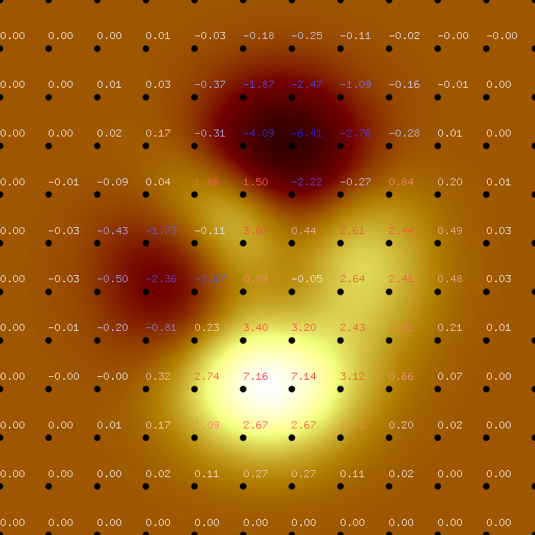
where r and c are the number of rows-1 or number of columns-1. Potential values are assigned in the figure below:
 This interpolation method is based on the bump function convolution.
For this reason, it becomes necessary to violate the control point values, so that the smoothmap generally differ from potential values assigned to the control points.
The violation is caused by the fact that the utilized convolution function is set to have a width larger than the grid width which is set to 1.
Note that the blue bump function spans five non-zero control points whereas the red spans six. The interpolation of coordinate q is obtained by:
This interpolation method is based on the bump function convolution.
For this reason, it becomes necessary to violate the control point values, so that the smoothmap generally differ from potential values assigned to the control points.
The violation is caused by the fact that the utilized convolution function is set to have a width larger than the grid width which is set to 1.
Note that the blue bump function spans five non-zero control points whereas the red spans six. The interpolation of coordinate q is obtained by:
 The following image shows three different simulations each containing two particles with different initial coordinates. The images on right show the motion in phase space for each of the three simulations. The non-dissipative nature of symplectic integrators allows for a accurate depictions of particles simulated over long time spans.
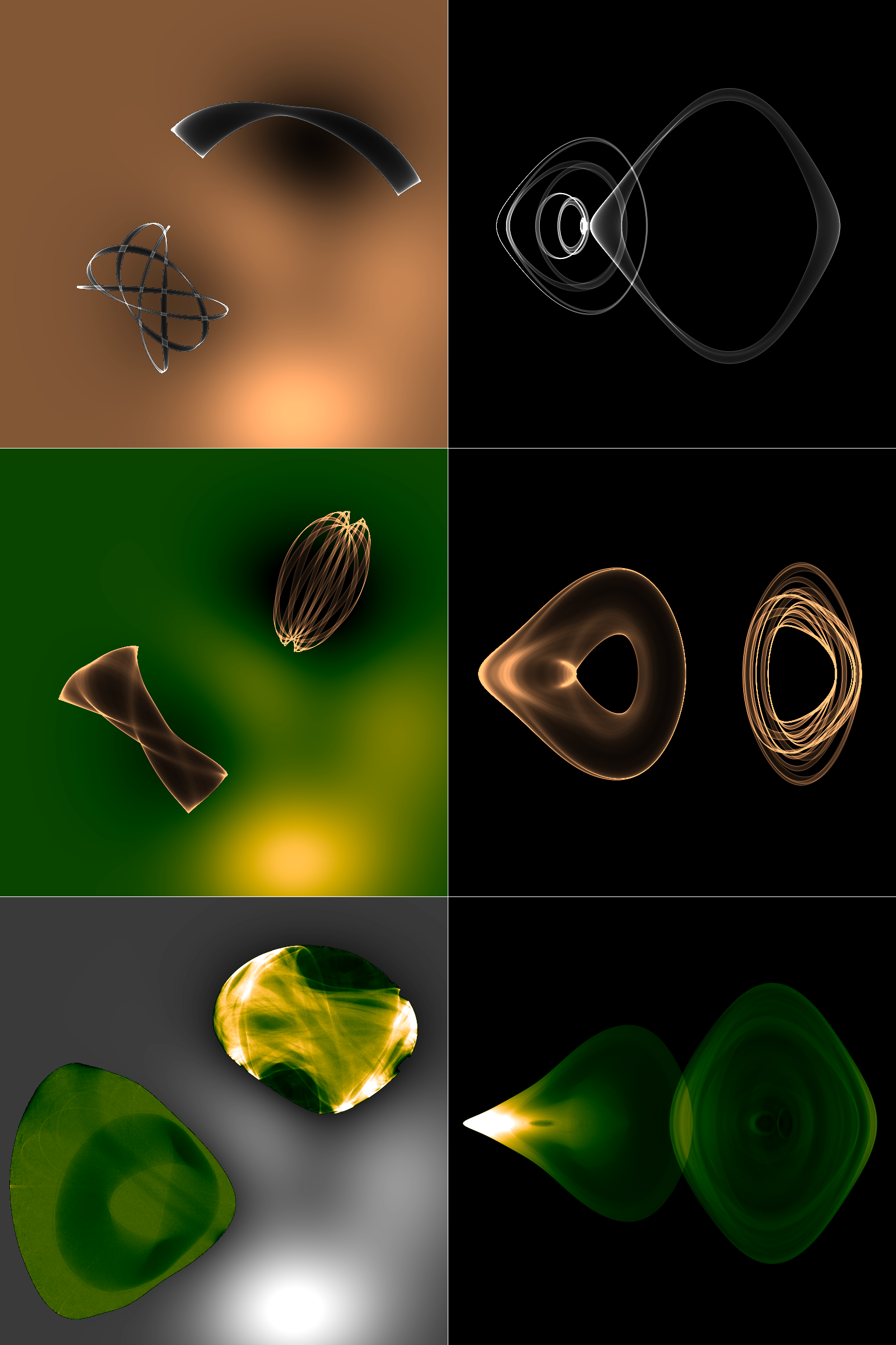 The time evolution of the particles exhibit rich dynamical behavior ranging from simple regular orbits to highly chaotic motions.
Analyses and discussions hereof remains to be discussed at a later time.
The time evolution of the particles exhibit rich dynamical behavior ranging from simple regular orbits to highly chaotic motions.
Analyses and discussions hereof remains to be discussed at a later time.
Method
Consider a two-dimensional potential grid. For simplicity we will consider the grid having integer coordinates:| (r,0) | (r,1) | (r,2) | ... | (r,c) |
| : | : | : | : | |
| (2,0) | (2,1) | (2,2) | ... | (2,c) |
| (1,0) | (1,1) | (1,2) | ... | (1,c) |
| (0,0) | (0,1) | (0,2) | ... | (0,c) |
\(\displaystyle{\qquad B(q,x)=exp \left( \frac{a(q-x)^2}{(q-x)^2-b^2} \right), (q-x)^2 \leq b^2 }\)
\(\displaystyle{\qquad B(q,x)=0, (q-x)^2 > b^2 }\)
where a and b are constants associated with the shape and the radius of the bump function respectively. The displacement of the bump function q along the first axis is associated with the position of the simulated particle.
The bump function has continuous derivatives of all orders. Consequently any convolution with the bump function is perfectly smooth in the sense of also having continuous derivatives of all orders.
Assuming an appropriate set of constants a and b, the bump function B(0,x) and B(1.6,x) is shown in the following figure.
\(\displaystyle{\qquad interp(q) = c \cdot \sum_{x} z(x) \cdot B(q,x) }\)
where c is a normalization constant and x is any integer for which B is non-zero. z(x) is not defined for x < 0 or x ≥ rows (or columns), in which case we may clamp the index. For example, we obtain the interpolated values at q = 0.0 and q = 1.6 by:
\(\displaystyle{\qquad interp(0.0) = c \cdot [z(0) \cdot B(0,-2) + z(0) \cdot B(0,-1) + z(0) \cdot B(0,0) + z(1) \cdot B(0,1) + z(2) \cdot B(0,2)] }\)
\(\displaystyle{\qquad interp(1.6) = c \cdot [z(0) \cdot B(1.6,-1) + z(0) \cdot B(1.6,0) + z(1) \cdot B(1.6,1) + z(2) \cdot B(1.6,2) + z(3) \cdot B(1.6,3) + z(4) \cdot B(1.6,4)] }\)
Coefficients a, b and c
a and b are constants associated with the bump function and are found by minimizing the difference between the minimum and maximum value of interp(q) given a constant potential assigned to all control points. It is worth noting that when the same potential is assigned to all control points, the smoothing method will only ever produce the same value at all q if the potential is 0. However, for non-zero potential the difference between the smallest and largest value of interp(q) decreases exponentially with additional evaluations on the bump function (increased value of b), which comes at the cost of additional computations. If two additional points are added to the bump function (b increased by 1), the gap decreases by approximately three orders of magnitude. We find the parameters b = 9.125638551411438 and c = 2.885628490404049 to be a pair of coefficients that minimizes the gap and provides a balanced smoothing width with a computational complexity of only 4 to 6 exponential function evaluations. c is a normalization constant found by minimizing the distance between interp(q) and a constant potential value assigned to all control points. Given values the values a and b above, the constant c is found to be a approximately 0.63450804436.Generalization of interp to higher dimensions
This smoothmap interpolation is extended to higher dimensions in the same way as spline methods. It is, however, noteworthy that the complexity of 2D splines is O(L) where L is the row or column length of the grid as opposed to 2D smoothmap interpolation which is O(constant), where this constant is related to 8-12 exponential function evaluations regardless of the grid size. The interpolated potential interp(q1,q2) is obtained by first evaluating interp(q2) at all control points in the first dimension where the bump function is non-zero. This produces 4 to 6 interpolated values, which are used as temporary control points for evaluating interp(q1). This logic is easily extended to higher dimensions n with a computational cost of O(bn) still far superior to the spline method O(Ln).Gradient evaluations
The gradient of B(q,x) along the first axis is obtained by first evaluating interp(q2) as mentioned in the previous section. The interpolated values are then used as temporary control points for evaluating grad(q1) using:
\(\displaystyle{\qquad grad(q) = \sum_{x} \frac{\partial B(q,x)}{\partial q} = \sum_{x} \frac{2ab^2(q-x)B(q,x)}{b^2-(q-x)^2} }\)
where x is any integer for which B is non-zero.
The gradient of B(q,x) along the second axis is similarly obtained by first evaluating interp(q1) for producing the control points required to obtain grad(q2).
Note that the gradient can be expressed in terms of B instead of exponential functions, which allows for more efficient implementation of gradient evaluations.
Results
An optimized implementation of the bump smoothmap is provided in "bump smoothmap.cpp". In this section we consider simulations of particles with various initial conditions using the following potential map://Part of "bump smoothmap.cpp" available with Zymplectic
double Grid[][12] = {
0, 0, 0, 0, 0, 0, 0, 0, 0, 0, 0, 0,
0, 0.0001, 0.0013, 0.0053,-0.0299,-0.1809,-0.2465,-0.1100,-0.0168,-0.0008,-0.0000, 0,
0, 0.0005, 0.0089, 0.0259,-0.3673,-1.8670,-2.4736,-1.0866,-0.1602,-0.0067, 0.0000, 0,
0, 0.0004, 0.0214, 0.1739,-0.3147,-4.0919,-6.4101,-2.7589,-0.2779, 0.0131, 0.0020, 0,
0,-0.0088,-0.0871, 0.0364, 1.8559, 1.4995,-2.2171,-0.2729, 0.8368, 0.2016, 0.0130, 0,
0,-0.0308,-0.4313,-1.7334,-0.1148, 3.0731, 0.4444, 2.6145, 2.4410, 0.4877, 0.0301, 0,
0,-0.0336,-0.4990,-2.3552,-2.1722, 0.8856,-0.0531, 2.6416, 2.4064, 0.4771, 0.0294, 0,
0,-0.0137,-0.1967,-0.8083, 0.2289, 3.3983, 3.1955, 2.4338, 1.2129, 0.2108, 0.0125, 0,
0,-0.0014,-0.0017, 0.3189, 2.7414, 7.1622, 7.1361, 3.1242, 0.6633, 0.0674, 0.0030, 0,
0, 0.0002, 0.0104, 0.1733, 1.0852, 2.6741, 2.6725, 1.1119, 0.1973, 0.0152, 0.0005, 0,
0, 0.0000, 0.0012, 0.0183, 0.1099, 0.2684, 0.2683, 0.1107, 0.0190, 0.0014, 0.0000, 0,
0, 0, 0, 0, 0, 0, 0, 0, 0, 0, 0, 0};
\(\displaystyle{\qquad H(\mathbf{p},\mathbf{q})=\frac{\mathbf{\mathbf{p}}^2}{2m}+m \cdot interp(q_1,q_2) }\)
where the mass m is set to 1 for convenience.
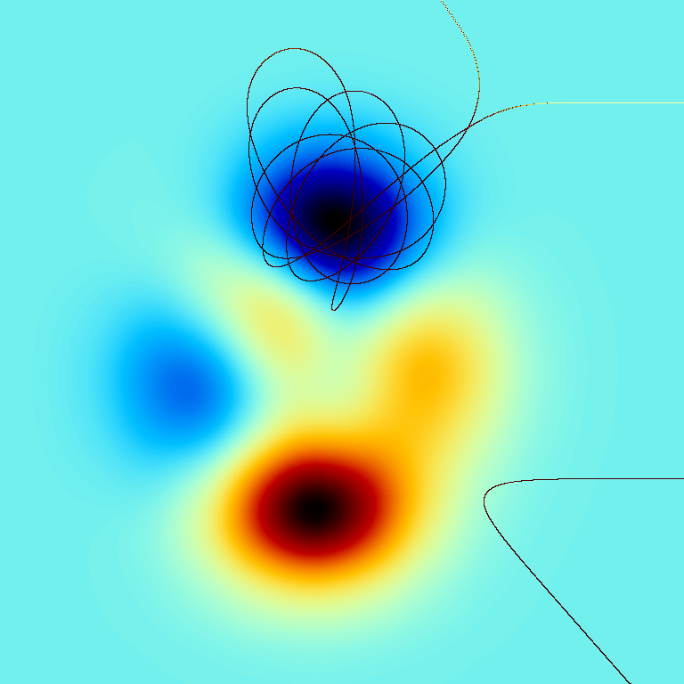
The following image shows the motion of two particles initialized on right moving left. The particles are likely to escape the region of interest because their Hamiltonian is larger than 0. This is confirmed by the trajectories of both particles.