Zymplectic project
Benchmark: Fifth order integrators
Performance of a family of fifth order explicit symplectic integrators is evaluated for various Hamiltonian systems.
Available with Zymplectic v.0.1.5
Coefficients of symplectic integrators satisfy series of equations, which approximates the time evolution of Hamiltonian systems up to a given order.
Some integrators are optimized for certain types of systems, although we will strictly discuss SPRK methods in these analyses.
It is possible to assign error estimates of integrators based on the coefficients alone, although practical implementations are necessary to test the performance (hereafter "benchmark") methods for any specific Hamiltonian system.
Applying the same time per evaluation for both methods, say 0.1 would imply that:
- The Euler method is iterated with τ = 0.1
- The third order method is iterated with τ = 0.3
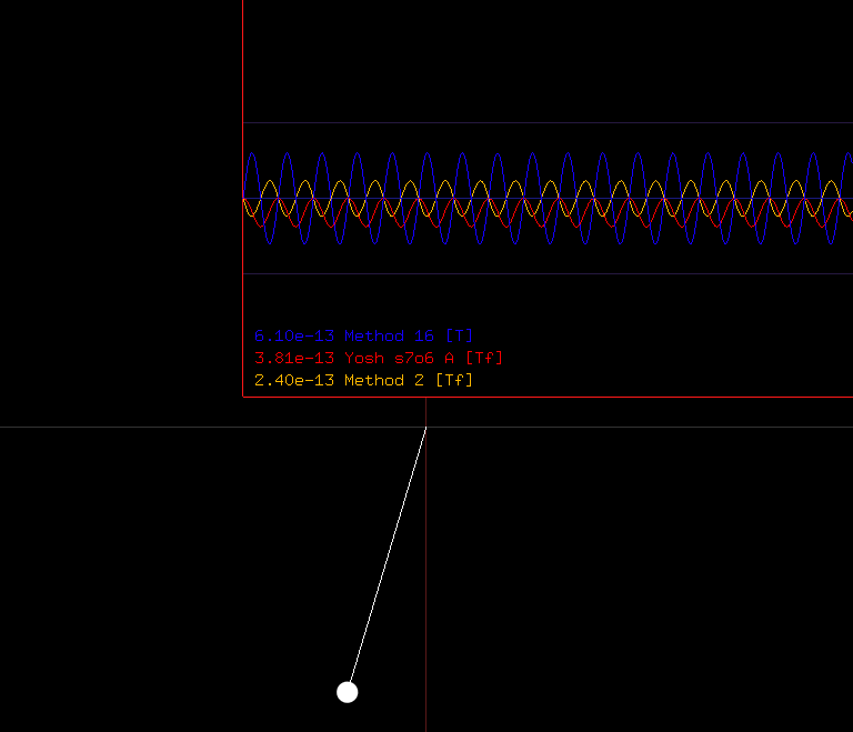
As visual context one may consider a cross section (see above graph) which depict a full simulation of each integrator at a given time step.
The error of these simulations are graphically displayed in Zymplectic during runtime.
The following figure displays error as a function of simulation time for each of the three methods with smallest maximum Hamiltonian deviation.
Defining "benchmark"
A benchmark provides a measure of accuracy per computational cost. By "accuracy" we associate either the relative or absolute error of the Hamiltonian:
\(\displaystyle{\qquad {\varepsilon _{rel}} = \frac{{\left| {H\left( t \right) - {H_0}} \right|}}{{|H_0|}} }\)
\(\displaystyle{\qquad {\varepsilon _{abs}} = \left| {H\left( t \right) - {H_0}} \right|}\)
where H0 is the initial Hamiltonian and H(t) is the Hamiltonian at a later time. A definite error can be assigned by either considering the maximum error or the average error over a time span long enough to properly represent the evolution of the system:
\(\displaystyle{\qquad {\varepsilon _{rel,max}} = \mathop {\max }\limits_{0 < t < {t_{end}}} \left( {\frac{{\left| {H\left( t \right) - {H_0}} \right|}}{{|H_0|}}} \right) }\)
\(\displaystyle{\qquad {\varepsilon _{rel,avg}} = \frac{1}{N}\sum\limits_{t = 0}^{{t_{end}}} {\left( {\frac{{\left| {H\left( t \right) - {H_0}} \right|}}{{|H_0|}}} \right)} }\)
where N is the number of iterations and H0 is assumed not to be 0. A definite absolute error can likewise be expressed.
By "computational cost" we associate the total number of gradient evaluations required to provide one time evolution of the canonical coordinates.
To compare the performance of integrators with different computational costs, it is neccessary to account for the different number of gradient evaluations.
We introduce the term "time per evaluation" which is a measure of the time progressed per computational cost or more precisely the time per pair of T and V gradient evaluations.
A complete analysis involve one of these error estimates evaluated for any time step τ
Example:
Consider a benchmark of the symplectic Euler method (c1=d1=1) and the rational third order integrator by Ruth 1983 (c1=1, c2=-2/3, c3=2/3, d1=-1/24, d2=3/4, d3=7/24).Applying the same time per evaluation for both methods, say 0.1 would imply that:
- The Euler method is iterated with τ = 0.1
- The third order method is iterated with τ = 0.3
Benchmarking fifth order integrators
We desire to test the performance of fifth order integrators published in "Tselios, Kostas and Simos, T. E.. Optimized fifth order symplectic integrators for orbital problems. Rev. mex. astron. astrofis. 2013, vol.49, n.1, pp.11-24. ISSN 0185-1101" and furthermore compare them with the acclaimed fourth order method "Ruth 1989" and sixth order method "Yosh s7o6 A". All fifth order methods are found in "integrators s7o5.zym". The best-performing "Method 2" is also found within the default integrator file "integrators.zym" under the name "Tselios5". The benchmarks are performed using the systems under default initial conditions distributed with Zymplectic:- The simple pendulum from "simple pendulum.cpp" performed using relative benchmark
- The two-body problem from "two-body central-force equivalence.cpp" (system 1 only) performed using relative benchmark
- The Kapitza pendulum from "Kapitza pendulum.cpp" performed using absolute benchmark
The simple pendulum
The following graph displays the average relative error of the Hamiltonian εrel,avg as a function of time per gradient pair evaluation. The graph is displayed in a log-log diagram depicting the integrator order as the slope of the lines. Note the distinctive slopes of the star- and triangle-marked lines in relation to the 4th and the 6th order integrators. It is noteworthy that the well-acclaimed 4th order method "Ruth 1989 [Tf]" is only competitive for large time steps whereas the well-acclaimed 6th order method "Yoshs7o6 A [Tf]" only performs better than the second fifth order method in the domain where the error approaches the limit of double-precision arithmetic. The naming conventations [T] refers to integrators where the gradient of T is evaluated first, whereas f in [Tf] refers to integrators with "first same as last" or "FSAL". FSAL implies that the last d-coefficient is zero and the computational cost of the integrator is reduced, which is also accounted for in the "time per evaluation" definition.