Zymplectic project
Integrator (autonomous and separable)
Implementations of the explicit symplectic integrator, specifically the SPRK-method for separable and autonomous Hamiltonian systems, are discussed and are described in terms of Octave/MATLAB code
We consider here the simplest case of explicit symplectic integrators where the Hamiltonian is separable and autonomous:
$$H(\mathbf{p},\mathbf{q}) = T(\mathbf{p}) + V(\mathbf{q})$$
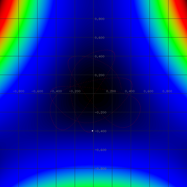
The implementations described in this section can be applied to a wide range of physical systems, but are here shown specifically for the Henon-Heiles system, which is expressed by:
$$T(\mathbf{p}) = \frac{1}{2}(p_1^2 + p_2^2)$$
$$V(\mathbf{q}) = \frac{1}{2}(q_1^2 + q_2^2) + \lambda(q_1^2 q_2 -\frac{q_2^3}{3})$$
where λ is here set to 1. The potential is visualized and first part of the simulation is shown below:
Symplectic euler (method 0)
As this method is not particularly accurate or useful, we list this method only as background of the methods to follow. The symplectic time evolution of the coordinates $$(q_{old},p_{old}) \rightarrow (q_{new},p_{new})$$ over the time step τ can be obtained by the symplectic Euler method: $$q_{new}=q_{old} + \tau\frac{\partial T}{\partial p}(p_{old})$$ $$p_{new}=p_{old} - \tau\frac{\partial V}{\partial q}(q_{new})$$ where q and p are interpreted as vectors in the multidimensional case. This procedure can be repeated any number of iterations without generating any dissipative error of the Hamiltonian even if the symplectic Euler method is only of first order. It should be noted that the time evolution is only symplectic if τ is reasonably small and the second derivatives of the Hamiltonian are smooth in the relevant area of integration.Vanilla explicit symplectic integrator (method 1)
Higher order explicit symplectic integrators are obtained by splitting the time evolution by multiple intermediate steps: $$q_{1}=q_{old} + \tau c_1\frac{\partial T}{\partial p}(p_{old}) $$ $$p_{1}=p_{old} - \tau d_1\frac{\partial V}{\partial q}(q_{1})$$ $$q_{2}=q_{1} + \tau c_2\frac{\partial T}{\partial p}(p_{1}) $$ $$p_{2}=p_{1} - \tau d_2\frac{\partial V}{\partial q}(q_{2})$$ $$q_{3}=q_{2} + \tau c_3\frac{\partial T}{\partial p}(p_{2}) $$ $$p_{3}=p_{2} - \tau d_3\frac{\partial V}{\partial q}(q_{3})$$ $$...$$ $$q_{new}=q_{s-1} + \tau c_{s}\frac{\partial T}{\partial p}(p_{s-1}) $$ $$p_{new}=p_{s-1} - \tau d_{s}\frac{\partial V}{\partial q}(q_{s})$$ where c and d are arrays containing the splitting coefficients which each sum up to 1, and s is the number of "stages" associated with the length of these arrays. The symplectic Euler method is considered a 1-stage integrator where c1=d1=1. It is important to note that only qnew, pnew, qold, pold are meaningful and that the intermediate steps provide no useful information about the time evolution. The algorithm is implemented in the following MATLAB code, which simulates the Henon-Heiles system and displays the Hamiltonian error as a function of time.% We consider the two-dimensional Hamiltonian system "Henon-Heiles"
% The Hamiltonian is separable and autonomous
lambda = 1.0;
Hamilton = @(p,q) (0.5*(p(1)^2+p(2)^2)+0.5*(q(1)^2+q(2)^2) + lambda*(q(1)^2*q(2)-q(2)^3/3));
dV = @(q) ([q(1)+2*lambda*q(1)*q(2), q(2)+lambda*(q(1)^2-q(2)^2)]); %Gradient of V
dT = @(p) ([p(1), p(2)]); %Gradient of P
% Integrator coefficients can be obtained from the text file "integrators.zym"
% The following coefficients "Ruth 1989" provide a 4-stage 4th order integrator
c(1) = 0.675603595979828817;
c(2) =-0.175603595979828817;
c(3) =-0.175603595979828817;
c(4) = 0.675603595979828817;
d(1) = 1.351207191959657634;
d(2) =-1.702414383919315268;
d(3) = 1.351207191959657634;
d(4) = 0;
dt = 0.01; %time step size also denoted tau or h in other literature
IterCount = 5000; %number of iterations
H = zeros(IterCount,1);
T = dt*(0:(IterCount-1));
q = [0.3 0.0];
p = [0.0 0.4];
H(1) = Hamilton(p(1,:),q(1,:)); %Initial Hamiltonian
for n = 1:IterCount
for i = 1:length(c)
q = q + c(i)*dt*dT(p);
p = p - d(i)*dt*dV(q);
end
H(n) = Hamilton(p,q);
end
plot(T,H - H(1)) %display graphically the error of the HamiltonianFirst-same-as-last ABA variant (method 2)
Method 1 has been implemented with coefficients containing a last d-coefficient, which is zero. This is a common attribute of splitting coefficients and provides an opportunity to reduce the computational cost by not just one but two gradient evaluations: The last evaluation "p = p - 0*dt*dV(q);" obviously becomes unnecessary, and the new last gradient evaluation dT(p) can be saved for the first evaluation of the next iteration as p remains unchanged from the last gradient evaluation: $$q_{1}=q_{old} + \tau c_1 FSAL$$ $$p_{1}=p_{old} - \tau d_1\frac{\partial V}{\partial q}(q_{1})$$ $$q_{2}=q_{1} + \tau c_2\frac{\partial T}{\partial p}(p_{1})$$ $$p_{2}=p_{1} - \tau d_2\frac{\partial V}{\partial q}(q_{2})$$ $$...$$ $$q_{s-1}=q_{s-2} + \tau c_s\frac{\partial T}{\partial p}(p_{s-2})$$ $$p_{new}=p_{s-2} - \tau d_s\frac{\partial V}{\partial q}(q_{s-1})$$ $$FSAL = \frac{\partial T}{\partial p}(p_{s-1})$$ $$q_{new}=q_{s-1} + \tau c_s FSAL$$ This is typically referred to as "first same as last" or "FSAL" and effectively reduces the computational cost of the integrator by one stage. The implementation of the FSAL-variant is shown below:lambda = 1.0;
Hamilton = @(p,q) (0.5*(p(1)^2+p(2)^2)+0.5*(q(1)^2+q(2)^2) + lambda*(q(1)^2*q(2)-q(2)^3/3));
dV = @(q) ([q(1)+2*lambda*q(1)*q(2), q(2)+lambda*(q(1)^2-q(2)^2)]);
dT = @(p) ([p(1), p(2)]);
c(1) = 0.675603595979828817; %"Ruth 1989"
c(2) =-0.175603595979828817;
c(3) =-0.175603595979828817;
c(4) = 0.675603595979828817;
d(1) = 1.351207191959657634;
d(2) =-1.702414383919315268;
d(3) = 1.351207191959657634; %c(4) is now undeclared and unused
dt = 0.01;
IterCount = 5000;
H = zeros(IterCount,1);
T = dt*(0:(IterCount-1));
q = [0.3 0.0];
p = [0.0 0.4];
H(1) = Hamilton(p(1,:),q(1,:));
FSAL = dT(p); %First same as last
for n = 1:IterCount
q = q + c(1)*dt*FSAL; %Calculated in the end of each step
p = p - d(1)*dt*dV(q);
for i = 2:(length(c)-1)
q = q + c(i)*dt*dT(p);
p = p - d(i)*dt*dV(q);
end
FSAL = dT(p); %Used at the beginning of next step
q = q + c(length(c))*dt*FSAL;
H(n) = Hamilton(p,q);
end
plot(T,H - H(1))Alternating ABA-BAB variant (method 3)
We have used a set of symmetric splitting coefficients in method 1 and 2. In case the the integrator coefficients are not symmetric, we can construct a more powerful integration scheme. First it must be established that all splitting coefficients can also be implemented in reversed form, meaning that if c and d are splitting coefficients, then calt and dalt are also splitting coefficients with the same properties: $$c_{alt} = reverse(d)$$ $$d_{alt} = reverse(c)$$ although the alternative integrator with calt and dalt need also to be implemented in the reversed form: $$p_{1}=p_{old} - \tau d_{alt,1}\frac{\partial V}{\partial q}(q_{old})$$ $$q_{1}=q_{old} + \tau c_{alt,1}\frac{\partial T}{\partial p}(p_{1})$$ $$p_{2}=p_{1} - \tau d_{alt,2}\frac{\partial V}{\partial q}(q_{1})$$ $$q_{2}=q_{1} + \tau c_{alt,2}\frac{\partial T}{\partial p}(p_{2})$$ $$...$$ Second, symplectic integrators can be concatenated without waiving symplectic properties. This means that one step can be performed with c and d while the next with calt and dalt. Third, we exploit that any integrator with symmetric splitting coefficients are always of even order. If we perform two iterations where the first is performed with c and d, and the second with calt and dalt, we are in fact using a symmetric composition, which effectively increases the order of accuracy from any odd order by one. This is achieved without any additional computational costs as shown in the implementation below where a third order integrator yields a fourth order accuracy:lambda = 1.0;
Hamilton = @(p,q) (0.5*(p(1)^2+p(2)^2)+0.5*(q(1)^2+q(2)^2) + lambda*(q(1)^2*q(2)-q(2)^3/3));
dV = @(q) ([q(1)+2*lambda*q(1)*q(2), q(2)+lambda*(q(1)^2-q(2)^2)]);
dT = @(p) ([p(1), p(2)]);
% The following coefficients provide a 3-stage 3rd order integrator
c(1) = 1;
c(2) =-2/3;
c(3) = 2/3;
d(1) =-1/24;
d(2) = 3/4;
d(3) = 7/24;
dt = 0.01;
IterCount = 5000;
H = zeros(IterCount,1);
T = dt*(0:(IterCount-1));
q = [0.3 0.0];
p = [0.0 0.4];
H(1) = Hamilton(p(1,:),q(1,:)); %Initial Hamiltonian
for n = 1:IterCount
if (mod(n,2) == 0) %Alternating between forward and backward implementation
for i = 1:length(d)
q = q + c(i)*dt*dT(p);
p = p - d(i)*dt*dV(q);
end
else
for i = length(d):-1:1
p = p - d(i)*dt*dV(q);
q = q + c(i)*dt*dT(p);
end
end
H(n) = Hamilton(p,q);
end
plot(T,H - H(1))FSAL-alternating variant (method 4)
An improved variant of method 3 can be composed in the same way as was done in method 2. Method 3 has a FSAL-component in both the beginning and the end of each iteration, which effectively reduces the computational cost by 1 stage. The FSAL-alternating variant is implemented below:lambda = 1.0;
Hamilton = @(p,q) (0.5*(p(1)^2+p(2)^2)+0.5*(q(1)^2+q(2)^2) + lambda*(q(1)^2*q(2)-q(2)^3/3));
dV = @(q) ([q(1)+2*lambda*q(1)*q(2), q(2)+lambda*(q(1)^2-q(2)^2)]);
dT = @(p) ([p(1), p(2)]);
% The following coefficients provide a 3-stage 3rd order integrator
c(1) = 1;
c(2) =-2/3;
c(3) = 2/3;
d(1) =-1/24;
d(2) = 3/4;
d(3) = 7/24;
dt = 0.01;
IterCount = 5000;
H = zeros(IterCount,1);
T = dt*(0:(IterCount-1));
q = [0.3 0.0];
p = [0.0 0.4];
H(1) = Hamilton(p(1,:),q(1,:)); %Initial Hamiltonian
FSAL = dT(p);
for n = 1:IterCount
if (mod(n,2) == 0) %Alternating between forward and backward implementation
q = q + c(1)*dt*FSAL;
p = p - d(1)*dt*dV(q);
for i = 2:(length(d)-1)
q = q + c(i)*dt*dT(p);
p = p - d(i)*dt*dV(q);
end
q = q + c(length(d))*dt*dT(p);
FSAL = dV(q);
p = p - d(length(d))*dt*FSAL;
else
p = p - d(length(d))*dt*FSAL;
q = q + c(length(d))*dt*dT(p);
for i = (length(d)-1):-1:2
p = p - d(i)*dt*dV(q);
q = q + c(i)*dt*dT(p);
end
p = p - d(1)*dt*dV(q);
FSAL = dT(p);
q = q + c(1)*dt*FSAL;
end
H(n) = Hamilton(p,q);
end
plot(T,H - H(1))