Spherical pendulum (stereographic projection)

The Hamiltonian of the spherical pendulum is derived using stereographic projection coordinates.
An implementation is presented and the advantages and disadvantages of this approach for dynamical systems is briefly discussed.

Available with Zymplectic v.0.4.1

The Hamiltonian of the spherical pendulum is presented most often in literature using Euler angles:

\(\displaystyle{\qquad H\left( {p,q} \right) = \frac{{p_2^2}}{{2m{r^2}\sin {{\left( {q_1} \right)}^2}}} + \frac{{p_1^2}}{{2m{r^2}}} + mgr\cos \left( {q_1} \right) }\)

In the following section, the Hamiltonian of the spherical pendulum will be derived using stereographic projection coordinates (SPC) yielding the Hamiltonian:

\(\displaystyle{\qquad H\left( {p,q} \right) = \frac{{p_1^2 + p_2^2}}{{2m{{\left( {\frac{{2r}}{{q_1^2 + q_2^2 + 1}}} \right)}^2}}} + gm\left( {r - \frac{{2r}}{{q_1^2 + q_2^2 + 1}}} \right) }\)

which is numerically far superior to the acclaimed Euler angle Hamiltonian as is discussed in the last section.

Defining the spherical pendulum

Define first the variables

• r as the constant length of the pendulum from the pendulum pivot to the bob
• m as the mass of the bob
• g is the gravitational constant

Additionally SPC are introduced to describe explicitly the Cartesian coordinates of the pendulum bob.

\(\displaystyle{\qquad \left( {x,y,z} \right) = r\left( {\frac{{2X}}{{1 + {X^2} + {Z^2}}},\frac{{ - 1 + {X^2} + {Z^2}}}{{1 + {X^2} + {Z^2}}},\frac{{2Z}}{{1 + {X^2} + {Z^2}}}} \right) }\)

where (x,y,z) is the position of the pendulum bob expressed in terms of the SPC (X,Z). More precisely, the point (X,Z) is the point of intersection of the xz-plane and the line defined by the north pole of the pendulum sphere and the pendulum bob. This is illustrated in the figure where the (X,Z) position is marked by the purple cylinder and the line from the north pole to the pendulum bob is shown in as the red line.

Deriving the Hamiltonian

The Cartesian coordinates (x,y,z) of the pendulum bob are retrieved directly from SPC, where the canonical coordinates q₁ and q₂ are defined as X and Z respectively.

\(\displaystyle{\qquad x = r\frac{{2{q_1}}}{{q_1^2 + q_2^2 + 1}} }\)

\(\displaystyle{\qquad y = r\frac{{ - 1 + q_1^2 + q_2^2}}{{1 + q_1^2 + q_2^2}} }\)

\(\displaystyle{\qquad z = r\frac{{2{q_2}}}{{q_1^2 + q_2^2 + 1}} }\)

where (q₁,q₂) is the projected position of the pendulum bob from the north pole through the pendulum bob and onto the xz-plane. Note that this projection is ill-defined at the north pole where both q₁ and q₂ approaches ∞ with sign that is also undefined. Hence numerical simulation near the north pole will produce increased error from compactness, significant truncation errors from coordinate scaling and a discontinuity under certain conditions.

Noting that q₁ and q₂ are functions of time, the Cartesian velocities are obtained directly as the time derivatives. The time derivatives can be simplified to:

\(\displaystyle{\qquad \dot x = {{\dot q}_1}a\left( {1 - \frac{{aq_1^2}}{r}} \right) - {{\dot q}_2}\frac{{{q_1}{q_2}{a^2}}}{r} }\)

\(\displaystyle{\qquad \dot y = \frac{{{a^2}}}{r}\left( {{q_1}{{\dot q}_1} + {q_2}{{\dot q}_2}} \right) }\)

\(\displaystyle{\qquad \dot z = {{\dot q}_2}a\left( {1 - \frac{{aq_2^2}}{r}} \right) - {{\dot q}_1}\frac{{{q_1}{q_2}{a^2}}}{r} }\)

where a is introduced for the sake of notational simplicity:

\(\displaystyle{\qquad a = \frac{{2r}}{{1 + q_1^2 + q_2^2}} }\)

the kinetic and potential energy are obtained:

\(\displaystyle{\qquad T = \frac{1}{2}m\left( {{{\dot x}^2} + {{\dot y}^2} + {{\dot z}^2}} \right) = \frac{1}{2}m\left( {\dot q_1^2 + \dot q_2^2} \right){a^2} }\)

\(\displaystyle{\qquad V = mgy = mg\left( {r - a} \right) }\)

from which the Lagrangian follows:

\(\displaystyle{\qquad L = T - V = \frac{1}{2}m\left( {\dot q_1^2 + \dot q_2^2} \right){a^2} - mg\left( {r - a} \right) }\)

yielding the canonical momenta:

\(\displaystyle{\qquad \frac{{\partial L}}{{{{\partial \dot q}_1}}} = p_1 = m{\dot q_1}{a^2} }\)

\(\displaystyle{\qquad \frac{{\partial L}}{{{{\partial \dot q}_2}}} = p_2 = m{\dot q_2}{a^2} }\)

The Hamiltonian can now by substitution be expressed explicitly in terms of the canonical coordinates p and q:

\(\displaystyle{\qquad H\left( {p,q} \right) = T + V = \frac{1}{{2m{a^2}}}\left( {p_1^2 + p_2^2} \right) + mg\left( {r - a} \right) }\)

Note that the Hamiltonian is nonseparable as it can not be separated into two functions T(p) and V(q). It is also worth noting that the Hamiltonian diverges at the north pole where a approaches 0 as either q₁ or q₂ approaches ∞

The system is simulated using the gradient of the Hamiltonian:

\(\displaystyle{\qquad \frac{{\partial H}}{{\partial p_1}} = \frac{p_1}{m a^2} }\)

\(\displaystyle{\qquad \frac{{\partial H}}{{\partial p_2}} = \frac{p_2}{m a^2} }\)

\(\displaystyle{\qquad \frac{{\partial H}}{{\partial q_1}} = q_1 b }\)

\(\displaystyle{\qquad \frac{{\partial H}}{{\partial q_2}} = q_2 b }\)

where

\(\displaystyle{\qquad b = \frac{{p_1^2 + p_2^2}}{{mra}} + \frac{{mg{a^2}}}{r} }\)

Implementation

The following code simulates the spherical pendulum. The pendulum is displayed in function DrawFunc by transforming the SPC to Cartesian coordinates. The pendulum bob trajectory is likewise displayed by function IterFunc.

//Copy-paste into Zymplectic or load as file to run the simulation
const double m = 1.0; //mass of the pendulum bob
const double r = 0.5; //pendulum length
const double g = 1.0; //gravitational constant

double H(Arg) {
	double a = 2*r/(q1*q1 + q2*q2 + 1); 
	return (p1*p1 + p2*p2)/(2*m*a*a) + g*m*(r - a);
}
void dH(Arg) {
	double a = 2*r/(q1*q1 + q2*q2 + 1);
	double b = (p1*p1 + p2*p2)/(m*r*a) + g*m*a*a/r;
	dq1 = q1*b;
	dq2 = q2*b;
	dp1 = p1/(m*a*a);
	dp2 = p2/(m*a*a);
}

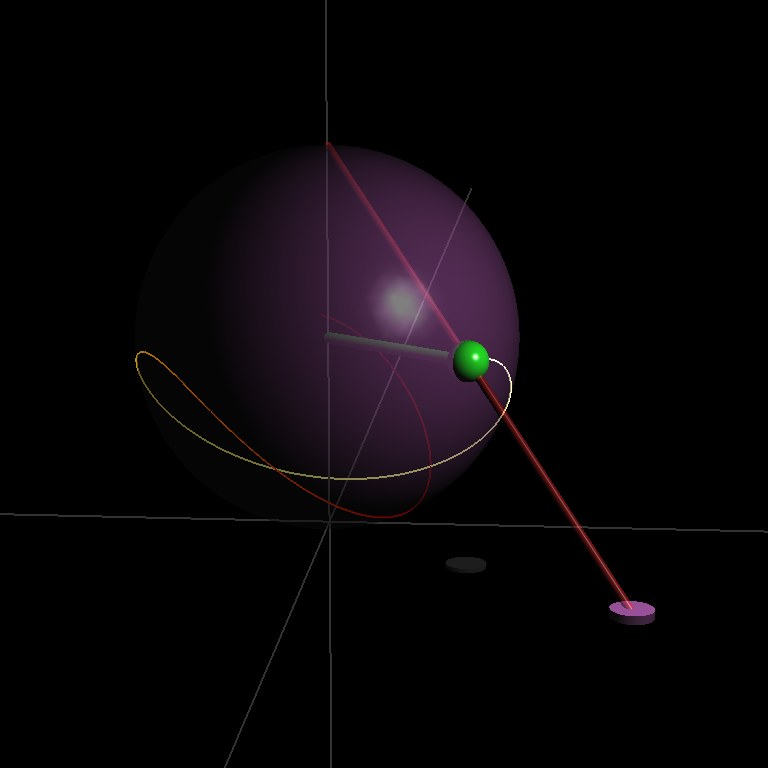
void DrawFunc() {
	double X = obj_q[0][0]; //X,Y is the projected position of the pendulum bob on the xz-plane
	double Z = obj_q[0][1];
	double a = 2*r/(X*X + Z*Z + 1);
	double x = a*X; //x,y,z is the actual position of the pendulum bob
	double y = 2*r - a;
	double z = a*Z;
	
	draw.rgb(0.1,0.8,0.1); 
	draw.sphere(x, y, z, 0.05);
	draw.rod(x, y, z, 0, r, 0, 0.015); 
	draw.rgb(0.1,0.1,0.1); draw.rod(x, 0, z, x, -0.01, z, 0.05); //projection onto z-plane
	draw.rgb(0.6,0.3,0.6); draw.rod(X, 0.01, Z, X, -0.01, Z, 0.05); //stereographic projection position
	draw.rgb(1,0.1,0.1,0.5); draw.rod(X, 0, Z, 0, 2*r, 0, 0.01);
	draw.rgb(0.6,0.3,0.6,0.5); draw.sphere(0,r,0,r);
}

void IterFunc() {
	double X = obj_q[0][0];
	double Z = obj_q[0][1];
	double a = 2*r/(X*X + Z*Z + 1);
	double x = a*X;
	double y = 2*r - a;
	double z = a*Z;
	
	draw.track_add(x, y); //display pendulum bob trajectory
	draw.trail(x, y, z);
}

double _q_init[] = {1, 0}; //initial position in the stereographic projection plane
double _p_init[] = {0, 0}; //initial momentum is set in main function

void main() {
	double dqx = 0; //(dqx,dqy) is the velocity in the stereographic projection plane
	double dqy = 1;
	double a = 2*r/(_q_init[0]*_q_init[0] + _q_init[1]*_q_init[1] + 1);

	_p_init[0] = dqx*m*a*a;
	_p_init[1] = dqy*m*a*a;

	Z.track = Z.trail = Z.graph3D = 1;
	Z.OnDraw = DrawFunc; //draw the pendulum
	Z.OnIter = IterFunc; //obtain bob trajectory

	Z.H(H,dH,0);
}

Discussion of stereographic projection for Hamiltonian systems

SPC provides a powerful way to derive and simulate Hamiltonian systems associated with spherical and rigid body motion. The spherical pendulum is the simplest SPC system among the example codes provided with Zymplectic. The major advantages and the few disadvantages of SPC can be summarized:

• The spherical pendulum in Euler angles can be simulated as a separable system unlike the SPC Hamiltonian that is strictly nonseparable. This means that the SPC simulation requires roughly twice as many evaluations.
• SPC has only one singularity, making it more feasible for simulating spherical systems than Euler angles that generally yield two singularities
• The SPC Hamiltonian of the spherical pendulum is rational unlike the Hamiltonian with Euler angles. This enables exact analytical and rational simulations of the spherical pendulum in phase space
• SPC is considerably more efficient for simulating the spherical pendulum as computationally expensive trigonometric functions are avoided. In fact, Zymplectic simulates the SPC roughly three times faster than the Euler angle spherical pendulum.
• The SPC Hamiltonian has low compactness at the south pole. This means that simulations where the pendulum is generally located near the south pole or just the southern hemisphere, generally produce Hamiltonian errors that are easily an order of magnitude smaller than the same simulation in Euler angles.
• The derivation of the Hamiltonian is generally equally difficult as with other coordinates. While the derivation is simple for the spherical pendulum, the complexity increases greatly for systems with more complicated expressions for the canonical momenta, even when the resulting Hamiltonian may be greatly simplified.

It is tempting to derive a Hamiltonian system with radial SPC such that

\(\displaystyle{\qquad \left( {x,y,z} \right) = r\left( {\frac{{2R\cos \theta }}{{1 + {R^2}}},\frac{{ - 1 + {R^2}}}{{1 + {R^2}}},\frac{{2R\sin \theta }}{{1 + {R^2}}}} \right) }\)

where the Hamiltonian is now expressed in terms of the SPC angle and radius, but this system produces the same compactness at the south pole as Euler angles.

There may be great benefits by simulating the system with complex SPC, but this remains to be explored at a later time.

Remarks

It is remarkable that neither the Hamiltonian or Lagrangian of the spherical pendulum in SPC are to be found in literature, even when the resulting Hamiltonian is simpler, without critical singularity and is computationally more efficient for simulations.