Spherical pendulum (Euler angles)

The Hamiltonian of the spherical pendulum is derived. An implementation is shown and various graphical results are presented.

Available with Zymplectic v.0.3.0 (revised from v.0.2.6)

The spherical pendulum is a simple three-dimensional dynamical system. The Hamiltonian of the spherical pendulum is derived and an implementation is shown to graphically present the the system in three dimensions.

Defining the spherical pendulum

Define first the variables

• r as the length of the pendulum from the pivot (origo) to the bob
• m as the mass of the bob
• θ is the angle between the z axis and the pendulum measured from top
• φ is the angle the pendulum measured from the positve x axis counterclockwise around the z-axis.
• g is the gravitational constant

The angles will be associated with the canonical coordinates q₁ = θ and q₂ = φ throughout this article.

Deriving the Hamiltonian

The Cartesian coordinates of the spherical pendulum are retrieved directly from the conventional definition of spherical coordinates.

\(\displaystyle{\qquad x = r\sin \left( {q_1} \right)\cos \left( {{q_2}} \right) }\)

\(\displaystyle{\qquad y = r\sin \left( {q_1} \right)\sin \left( {{q_2}} \right) }\)

\(\displaystyle{\qquad z = r\cos \left( {q_1} \right) }\)

although it must be assumed for numerical treatment that q₂ can assign any value as opposed to the conventional definition of spherical coordinates θ ∈ [0,π]. Noting that both q₁ and q₂ are functions of time, the time derivatives of the Cartesian coordinates are then:

\(\displaystyle{\qquad \dot x = {{\dot q}_1}r\cos \left( {q_1} \right)\cos \left( {{q_2}} \right) - {{\dot q}_2}r\sin \left( {q_1} \right)\sin \left( {{q_2}} \right) }\)

\(\displaystyle{\qquad \dot y = {{\dot q}_1}r\cos \left( {q_1} \right)\sin \left( {{q_2}} \right) + {{\dot q}_2}r\sin \left( {q_1} \right)\cos \left( {{q_2}} \right) }\)

\(\displaystyle{\qquad \dot z = - {{\dot q}_1}r\sin \left( {q_1} \right) }\)

the kinetic and potential energy are obtained:

\(\displaystyle{\qquad T = \frac{1}{2}m\left( {{{\dot x}^2} + {{\dot y}^2} + {{\dot z}^2}} \right) = \frac{1}{2}m{r^2}\left( {\dot q_2^2\sin {{\left( {q_1} \right)}^2} + \dot q_1^2} \right) }\)

\(\displaystyle{\qquad V = mgz = mgr\cos \left( {q_1} \right) }\)

from which the Lagrangian follows:

\(\displaystyle{\qquad L = T - V = \frac{1}{2}m{r^2}\left( {\dot q_2^2\sin {{\left( {q_1} \right)}^2} + \dot q_1^2} \right) - mgr\cos \left( {q_1} \right) }\)

yielding the canonical momenta:

\(\displaystyle{\qquad \frac{{\partial L}}{{{{\partial \dot q}_1}}} = p_1 = m{{\dot q}_1}{r^2} }\)

\(\displaystyle{\qquad \frac{{\partial L}}{{{{\partial \dot q}_2}}} = p_2 = m{{\dot q}_2}{r^2} sin(q_1)^2 }\)

The Hamiltonian can now be expressed explicitly in terms of the canonical coordinates p and q:

\(\displaystyle{\qquad H\left( {p,q} \right) = T + V = \frac{{p_2^2}}{{2m{r^2}\sin {{\left( {q_1} \right)}^2}}} + \frac{{p_1^2}}{{2m{r^2}}} + mgr\cos \left( {q_1} \right) }\)

Note that the Hamiltonian seems nonseparable as it can not be separated into two functions T(p) and V(q). It is also worth noting that the Hamiltonian diverges at the poles q₁ = 0 and q₁ = π The poles should never be occupied for a spherical pendulum with non-zero rotational velocity around the z-axis.

\(\displaystyle{\qquad \frac{{\partial H}}{{\partial {p_1}}} = \frac{p_1}{{m r^2}} }\)

\(\displaystyle{\qquad \frac{{\partial H}}{{\partial {p_2}}} = \frac{p_2}{{m r^2 \sin {{\left( {q_1} \right)}^2}}} }\)

\(\displaystyle{\qquad \frac{{\partial H}}{{\partial q_1}} = - \frac{{p_2^2\cos \left( {q_1} \right)}}{{m r^2\sin {{\left( q_1 \right)}^3}}} - mgr\sin \left( {q_1} \right) }\)

\(\displaystyle{\qquad \frac{{\partial H}}{{\partial {q_2}}} = 0 }\)

The last terms being zero implies that p₂ must be constant. More precisely, p₂ is constant because this is associated with the angular momentum of the spherical pendulum. It follows from p₂ being constant that the Hamiltonian is separable:

\(\displaystyle{\qquad T = \frac{{p_1^2}}{{2m{r^2}}} }\)

\(\displaystyle{\qquad V = \frac{{p_2^2}}{{2m{r^2}\sin {{\left( {{q_1}} \right)}^2}}} + mgr\cos \left( {{q_1}} \right) }\)

Following should be noted on the separable form:

• The potential V is commonly associated with the effective potential.
• The separable form is governed by the same equations of motions when accounting for p₂ being constant.
• The spherical pendulum can be simulated using only the time evolution of q₁ and p₁. In this case, q₂ must be obtained by other means to graphically the cyclic rotation of the pendulum

Implementation

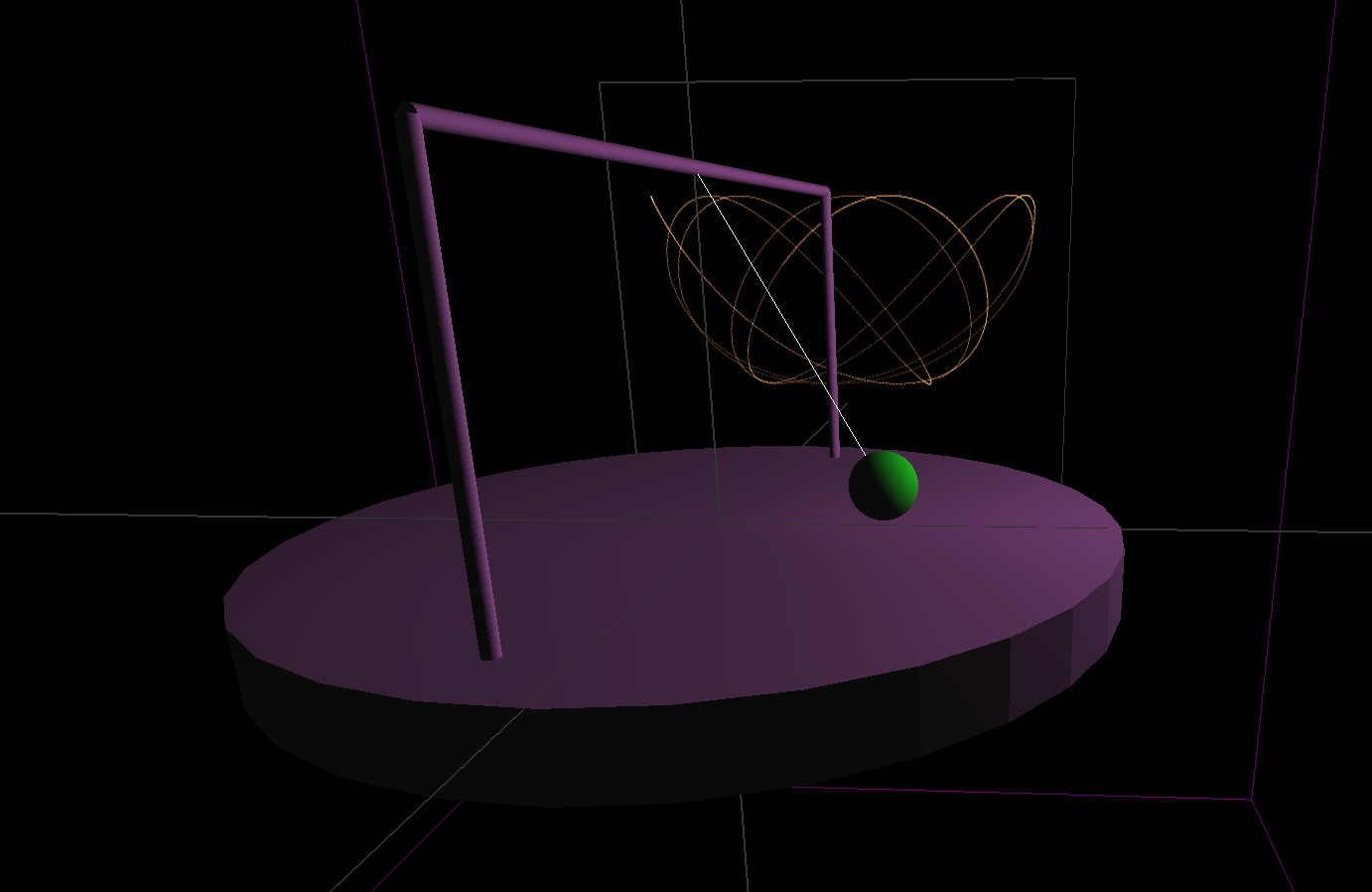
The following code simulates the spherical pendulum. The pendulum is displayed in function DrawFunc by transforming q₁ and the time tau to Cartesian coordinates. The pendulum bob trajectory is displayed by function IterFunc. Disabling DrawFunc will display the angle coordinates in the phase space, and allows energy surface display as presented in results.

//Copy-paste into Zymplectic or load as file to run the simulation
#include "math.h"
const double m = 1.0; //mass of the pendulum bob
const double w1 = 0.0; //initial angular velocity in relation to the latitude
const double w2 = 1.0; //initial angular velocity around z-axis
const double r = 0.5; //pendulum length
const double g = 1.0; //gravitational constant

double V(Arg) {
	return p2*p2/(2*m*r*r*sin(q1)*sin(q1)) + m*g*r*cos(q1);
}
double T(Arg) {
	return p1*p1/(2*m*r*r);
}

void dV(Arg) {
	d1 = -p2*p2*cos(q1)/(m*r*r*sin(q1)*sin(q1)*sin(q1)) - m*g*r*sin(q1);
	d2 = 0.0;
}
void dT(Arg) {
	d1 = p1/(m*r*r);
	d2 = p2/(m*r*r*sin(q1)*sin(q1));
}

void DrawFunc() {
	double x = r*sin(obj_q[0][0])*cos(obj_q[0][1]);
	double y = r*sin(obj_q[0][0])*sin(obj_q[0][1]);
	double z = r*cos(obj_q[0][0]);
	double GX[2] = {x,0};
	double GY[2] = {z + r,r}; //depicting x,z rather than x,y
	double GZ[2] = {y,0};

	draw.light(2*r,r,0,1);
	draw.lines(GX,GY,GZ,2);
	draw.rgb(0.1,0.8,0.1,1);
	draw.sphere(GX[0], GY[0], GZ[0], 0.05);
	draw.rgb(0.6,0.3,0.6,1);	
	draw.rod(0, -0.1, 0, 0, 0, 0, r*1.2, obj_q[0][1], 32); //make platform
	double c = -r*sin(obj_q[0][1]), s = r*cos(obj_q[0][1]);
	draw.rod(c, 0, s, c, r, s, 0.01); //make bipod
	draw.rod(-c, 0, -s, -c, r, -s, 0.01);
	draw.rod(c, r, s, -c, r, -s, 0.01);
}

void IterFunc() {
	double x = r*sin(obj_q[0][0])*cos(obj_q[0][1]);
	double y = r*cos(obj_q[0][0]);
	draw.track_add(x, y + r); //display pendulum bob trajectory
}

double _q_init[2] = {-1.5,0}; //initial latitude (undefined at the poles 0 and pi) and longitude
double _p_init[2] = {0,0};

void main() {
	Z.tstep = 0.0005;

	_p_init[0] = m*w1*r*r; //calculate p1 from the initial angular velocity w2
	_p_init[1] = m*w2*r*r*sin(_q_init[0])*sin(_q_init[0]); //calculate p2 from the initial angular velocity w2

	Z.graph3D = 1;
	Z.OnDraw = DrawFunc; //draw the pendulum
	Z.OnIter = IterFunc; //obtain bob trajectory
	Z.track = 0;
	Z.amp = 10;
	Z.delay = 5;
	Z.xmin = 40; Z.ymin = 40; Z.zmin = 40; Z.xmax = 0.1125; Z.ymax = 0.5; Z.zmax = 1.75; //Camera
	Z.T(T,dT,0);
	Z.V(V,dV,0);
}

Spherical pendulum with solid platform

In the previous section, the spherical pendulum was graphically depicted as pendulum with one degree of freedom that was mounted to a massless rotating platform as illustrated in the following figure:

In extension to the previous derivation assume, without loss of generality, that the platform has a non-zero mass M and the mass of the bipod is neglected. The kinetic and potential is then:

\(\displaystyle{\qquad T = \frac{1}{2}m{r^2}\left( {\dot q_2^2\sin {{\left( {q_1} \right)}^2} + \dot q_1^2} \right) + \frac{1}{2}I\dot q_2^2 }\)

\(\displaystyle{\qquad V = mgr\cos \left( {q_1} \right) }\)

The canonical momenta can be obtained from the Lagrangian:

\(\displaystyle{\qquad \frac{{\partial L}}{{{{\partial \dot q}_1}}} = {p_1} = m{{\dot q}_1}{r^2} }\)

\(\displaystyle{\qquad \frac{{\partial L}}{{{{\partial \dot q}_2}}} = {p_2} = {{\dot q}_2}\left( {I + m{r^2}\sin {{\left( {{q_1}} \right)}^2}} \right) }\)

and are used to express the kinetic and potential energy:

\(\displaystyle{\qquad T = \frac{{p_1^2}}{{2m{r^2}}} }\)

\(\displaystyle{\qquad V = \frac{{p_2^2}}{{2\left( {I + m{r^2}\sin {{\left( {{q_1}} \right)}^2}} \right)}} + mgr\cos \left( {{q_1}} \right) }\)

from which the Hamiltonian gradient follows:

\(\displaystyle{\qquad \frac{{\partial T}}{{\partial {p_1}}} = \frac{{{p_1}}}{{m{r^2}}} }\)

\(\displaystyle{\qquad \frac{{\partial T}}{{\partial {p_2}}} = \frac{{{p_2}}}{{I + m{r^2}\sin {{\left( {{q_1}} \right)}^2}}} }\)

\(\displaystyle{\qquad \frac{{\partial V}}{{\partial {q_1}}} = - mr\frac{{g\sin \left( {{q_1}} \right) + 2p_2^2r\sin \left( {2{q_1}} \right)}}{{4{{\left( {I + m{r^2}\sin {{\left( {{q_1}} \right)}^2}} \right)}^2}}} }\)

\(\displaystyle{\qquad \frac{{\partial V}}{{\partial {q_2}}} = 0 }\)

Using zero moment of inertia (zero platform mass) reduces effectively the system to the spherical pendulum derived in the first section. The code for this system is implemented as an example in Zymplectic.

Remarks

It should be noted in particular that the spherical pendulum described in this article does not exhibit any chaotic trajectories regardless of initial conditions and platform mass.