Construction of the quadrupole mass spectrometer

The QMS is constructed by four parallel cylindrical ideally hyperbolic) rod electrodes as shown in the following figure: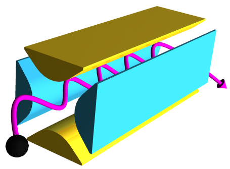 each pair of opposing electrodes is applied with a direct current u and an alternating current v with opposing polarity. At any given time the potential can be visualized as a saddle-surface. It can be shown that:

• the forces on the charged particle in the longitudinal direction (z-direction) are always zero.
• charged particles can be trapped in the xy-direction (stable motion) if u, v and the alternating current frequency ω are correctly chosen.
• charged particles of different masses are guided or trapped in the QMS for different values of u and v, allowing mass identification by detection of the charged particle throughput.

A motion of any particle with charge e and mass m inside the QMS is governed by the separable and non-autonomous Hamiltonian: $$H(\mathbf{p},\mathbf{q}) = T\left( \mathbf{p} \right) + V\left(\mathbf{q},t \right)$$ $$V\left( {{q_x},{q_y},t} \right) = \left( q_x^2 - q_y^2 \right)\frac{{u + v\cos(\omega t)}}{r_0^2}e$$ $$T\left( {{p_x},{p_y}} \right) = \frac{1}{2m} (p_x^2 + p_y^2)$$ with the gradient: $$\nabla H\left( {{q_x},{q_y},{p_x},{p_y}} \right) = \left\{ {\begin{array}{*{20}{c}} {2{q_x}\frac{{u + v\cos \left( {\omega t} \right)}}{{r_0^2}}}e\\ { - 2{q_y}\frac{{u + v\cos \left( {\omega t} \right)}}{{r_0^2}}}e\\ {{p_x}{m^{ - 1}}}\\ {{p_y}{m^{ - 1}}} \end{array}} \right.$$ where u and v are the DC-voltage and the radio-frequency voltage (RF-voltage) applied to the two pairs of electrodes and r₀ is the distance between the center and the surface of the hyperbolic rods. Note that physicists typically use φ as the electric potential where qφ=V and q is the electric charge which is here simply denoted as an electron charge e to avoid confusion with the canonical position coordinate. The Hamiltonian system associated with the QMS is non-autonomous because V depends explicitly on time. This implies that H in the general case is not preserved. A more detailed description of the QMS and the physical parameters is given in An Introduction to Quadrupole Ion Trap Mass Spectrometry. March, Raymond E. 4, 1997, Journal of mass spectrometry, Vol. 32, pp. 351-369.

The motion of a charged particle is a stable trajectory if an appropriate set of voltages are applied to the QMS electrodes. A stable trajectory is illustrated below as a particle hovering the electric potential surface in the QMS cross section.

The QMS allows distinction between different masses because particles because heavier or lighter particles may diverge and escape the QMS for a given set of electrode voltages. The parameters a and q are introduced as stability parameters and are associated with the stability of the particle motion within the QMS: $$a \equiv \frac{8e}{{m{{\left( {{r_0}\omega } \right)}^2}}}u$$ $$q \equiv \frac{4e}{{m{{\left( {{r_0}\omega } \right)}^2}}}u$$ assuming that the particle charge is e. The region of stable trajectories spanned by a and q can be obtained numerically (Mathieu stablity regions). The first stability region can be illustrated in the following diagram: The following video illustrates both stable and unstable motions of charged particles inside the QMS, and provides visual aid in understanding how the QMS may be utilized for mass spectrometry.

Implementation in Zymplectic

The system is implemented as any separable system. Zymplectic automatically detects the system as a non-autonomous system because the time "tau" is used in code. The following code simulates the motion of a single particle in the QMS.

//Copy-paste into Zymplectic or load as file to run the simulation
#include "math.h"
const double r0 = 0.01; //QMS inscribed radius [meter]
const double w = 8e+006; //QMS oscillation frequency [per second]
const double e = -1.0; //electric charge [electron charges]
const double mass_chlorine = 3.624266025057571e-007; //mass of the Cl-35 isotope [eV], calculated as 34.96885268*931494061/c^2
const double a_stability = 0.1; //Dimensionless constants which determine the system stability (See Mathieu stability diagram)
const double q_stability = 0.5;
double u,v,m; //set in initialization

double _q_init[] = {-0.008,0.004}; //Initial conditions do not influence the trajectory stability
double _p_init[] = {0.0,0.0};

double energy_V(Arg) {
	return (q1*q1 - q2*q2)*(u + v*cos(w*tau))/(r0*r0)*e; //depends explicitly on time (tau)
}
void dVdq(Arg) {
	d1 = q1*2.0*e/(r0*r0)*(u + v*cos(w*tau));
	d2 =-q2*2.0*e/(r0*r0)*(u + v*cos(w*tau));
}
double energy_T(Arg) {
    return 0.5*(p1*p1 + p2*p2)/m;
}
void dTdp(Arg) {
    d1 = p1/m;
    d2 = p2/m;
}

void main() { //this function is launched when executing script (Must be last function in file and not closed)
	Z.benchmark_time = 1e-5;
	Z.time_per_evaluation = 1e-9;
	Z.delay = 10;
	Z.energy_surface = 1;
	Z.V(energy_V,dVdq,0);
	Z.T(energy_T,dTdp,0);
	
	m = 1.0*mass_chlorine;
	u = a_stability*(mass_chlorine*r0*r0*w*w)/(-8.0*e);
	v = q_stability*(mass_chlorine*r0*r0*w*w)/(4.0*e);
}

Non-symplectic versus symplectic methods

Personal remarks

I am not aware of previous studies that have examined the QMS using explicit symplectic integrators. It is remarkable how well these integrators perform for this system in comparison to non-symplectic integrators.